TECHNICAL NOTEBOOK · CREATIO

Kinematic and dynamic analysis

From defining shape to predicting motion. A place to collect the formulation, physical assumptions and research results.

Five documented studies: CT–01, CT–02, EN–01, EN–02 and EN–02R. Each includes a synthesis distinguishing derived results, numerical checks and model limitations. Interactive tools and comparative views are identified separately.

01 · Foundations

Common mathematical definitions and modelling assumptions.

CT–01 · TECHNICAL NOTE

Mathematical formulation

CT–01 · Analytical

Study synthesis

Objective: Formalize the surface and distinguish geometry, pattern motion and mass motion.
Method: Original parametrization, chain-rule derivatives and an initial Lagrangian formulation.
Results obtained: Position, velocity, acceleration, normal and pattern angular velocity were derived: α̇p = −φ̇ₐ/Kₐ. The formulation separates prescribed geometry from dynamic transport.
Scope and limitations: The formulation does not establish that a mass follows a cavity. EN–02 and EN–02R extend the initial point-mass model to a sphere with finite radius, inertia and friction.

Version 0.1 · 19 September 2026 · Preliminary formulation for review

This note organizes the CREATIO parametrization and proposes an initial analysis framework. Kinematic relations follow from the chain rule; the dynamic model below approximates a point mass on a surface with prescribed motion.

1. Geometry and parameters

The CREATIO surface is described by the Cartesian parameterization $c (α, R, t)$ . The parameter $R$ measures distance from the inner radius in the reference surface; $α$ is the angular coordinate and $t$ denotes time.

0 < R_{0} < R_{1}, Δ R = R_{1} - R_{0}

R \in [0, Δ R], α \in [0, 2 π]

A \geq 0, K_{r}, K_{a} \in N_{>0}, t \geq 0

The wave profile combines radial and angular components:

W (α, R, t) = A \sin (\frac{2 π K_{r} R}{Δ R} + φ_{r} (t)) \cos (K_{a} α + φ_{a} (t))

(1)

The inclination $γ (t)$ transforms the radial–vertical plane. Defining the projected radius:

ρ (α, R, t) = R_{0} + R \cos (γ (t)) - W (α, R, t) \sin (γ (t))

(2)

c (α, R, t) = (\begin{array}{c} ρ (α, R, t) \cos (α) \\ ρ (α, R, t) \sin (α) \\ R \sin (γ (t)) + W (α, R, t) \cos (γ (t)) \end{array})

(3)

In the reference case $γ \equiv 0$ , this reduces to:

c (α, R, t) = (\begin{array}{c} (R_{0} + R) \cos (α) \\ (R_{0} + R) \sin (α) \\ W (α, R, t) \end{array})

(4)

$A$ is the amplitude; $K_{r}$ and $K_{a}$ are the radial and angular cycle counts. The phases $φ_{r} (t)$ and $φ_{a} (t)$ and the inclination $γ (t)$ are real-valued functions of time. All angles in the equations are in radians. The visualization controls display degrees and convert them internally.

Angular periodicity follows from $K_{a} \in N_{>0}$ : $α = 0$ and $α = 2 π$ represent the same position. The inclined family uses $- \frac{π}{2} \leq γ (t) \leq \frac{π}{2}$ .

In the animation, a phase can vary linearly, while inclination can oscillate sinusoidally:

φ_{a} (t) = φ_{a} (0) + ω t

(5)

γ (t) = γ_{0} + G \sin (Ω t)

(6)

Here, $ω$ is the phase rate, $Ω$ the oscillation angular frequency and $G$ its nonnegative angular amplitude, with $| γ_{0} | + G \leq \frac{π}{2}$ . The radial phase can follow the same linear law. These models describe geometric evolution, rather than contact forces.

2. Surface regularity and orientation

The parametrization is assumed twice continuously differentiable over the analysis domain. At regular points, the unit normal is defined by:

n = \frac{c_{α} \times c_{R}}{‖ c_{α} \times c_{R} ‖}, ‖ c_{α} \times c_{R} ‖ > 0

(7)

The α and R subscripts denote partial derivatives. The normal can be reversed to point towards the side accessible to the mass. Local regularity, absence of self-intersections and deformation limits must be checked for each parameter set.

3. Kinematics: surface, pattern and mass

Let q = (α, R) and the trajectory x(t) = c(q(t), t). Below, q₁ = α and q₂ = R; repeated indices i, j denote sums from 1 to 2. Partial time derivatives hold q fixed.

\dot{x} = c_{t} + c_{i} \dot{q_{i}}

(8)

\ddot{x} = c_{tt} + 2 c_{ti} \dot{q_{i}} + c_{ij} \dot{q_{i}} \dot{q_{j}} + c_{i} \ddot{q_{i}}

(9)

Here cᵢ = ∂c/∂qᵢ, cᵢⱼ = ∂²c/(∂qᵢ∂qⱼ), cₜᵢ = ∂²c/(∂t∂qᵢ) and cₜₜ = ∂²c/∂t². Dots on q denote total time derivatives. The velocity cₜ describes the parametrization at fixed coordinates; it equals membrane material velocity only if these coordinates label material points.

For constant Kₐ and a constant angular phase of the pattern, Kₐαₚ + φₐ(t) = constant, one obtains:

{\dot{α}}_{p} = - \frac{\dot{φ_{a}}}{K_{a}}

(10)

This is the angular velocity of the phase pattern. It does not determine a sphere’s speed or guarantee that it follows a cavity. Its trajectory depends on initial conditions, forces and contact.

4. Initial dynamic model

Assumptions: inertial frame; prescribed surface; constant point mass m; maintained contact in a regular region; ideal normal reaction. Load-induced membrane deformation and actuator dynamics are excluded from this first approximation.

T = \frac{m}{2} {‖ c_{t} + c_{i} \dot{q_{i}} ‖}^{2}, L = T - V

(11)

\frac{d}{d t} (\frac{\partial L}{\partial \dot{q_{i}}}) - \frac{\partial L}{\partial q_{i}} = Q_{i}

(12)

V(q,t) is potential energy evaluated on the surface. Qᵢ = fₙ꜀ · cᵢ is the nonconservative generalized force. For ideal frictionless sliding with no other nonconservative forces, Qᵢ = 0. In uniform gravity, V = −m g · c. Because the surface moves, the mass’s mechanical energy is generally not conserved: actuation performs work.

m \ddot{x} = m g + N n + f_{τ}, N \geq 0

(13)

Here N is the normal reaction and fτ is the tangential contact force; only gravity and contact are included. If the solution requires N < 0, unilateral contact is no longer admissible and separation must be handled. A finite-radius sphere requires an offset surface for its centre, rotational inertia and a friction/rolling law: the sphere centre is not identified with c.

5. Aerospace extension

\dot{H_{O}} = τ_{ext,O}

(14)

Hₒ is total angular momentum and τext,O is external torque, both about an origin O fixed in an inertial frame. The full system must include structure, membrane, actuators and moving masses. With zero external torque, Hₒ is conserved; internal motion can redistribute angular momentum and change orientation. Attitude prediction requires a coupled model, beyond the geometric animation.

In microgravity, the mechanism maintaining mass contact must be specified — for example, mechanical confinement or a modelled magnetic interaction. The assumptions in this note are working proposals, not CREATIO validation results.

02 · Kinematics

Geometry, derivatives, regularity and prescribed pattern motion.

CT–02 · SPATIAL KINEMATICS

From surface to kinematic space

CT–02 · Analytical + numerical verification

Study synthesis

Objective: Characterize the continuous geometric family from γ = 0° to 90°.
Method: Analytical derivatives, phase trajectories and helical pitch; finite differences at 19 inclinations, with 12,960 samples per step and additional time-varying γ cases.
Results obtained: The same equation describes an annulus, corrugated conical surfaces and the cylindrical limit. J ≥ 0.50 u was proved for the studied parameters. Finite differences show second-order convergence; maximum feature-velocity error was 3.74 × 10⁻¹² u/s.
Scope and limitations: Local regularity does not prove global absence of self-intersections. Phase trajectories are not sphere dynamics. u denotes a model length unit.

The original CREATIO equation defines a continuous geometric family. Here only γ varies from 0° to 90°; the reduced amplitude and all other parameters remain fixed. This chapter extends CT–01 without replacing its formulation or the existing numerical studies.

γ 0°

R₀ = 0.68 u · ΔR = 1.72 u · A = 0.18 u · Kᵣ = 1 · Kₐ = 6 · φᵣ = 0 · φₐ = 29°

1 · Original mapping and geometric limits

ΔR = R₁ − R₀, k = 2πKᵣ/ΔR, u = kR + φᵣ(t), v = Kₐα + φₐ(t)

W = A sin u cos v
ρ = R₀ + R cos γ − W sin γ
c(α,R,t) = (ρ cos α, ρ sin α, R sin γ + W cos γ)

Domain: R ∈ [0, ΔR], α ∈ [0, 2π), γ ∈ [0, π/2], R₀ > 0, ΔR > 0 and A ≥ 0. Kₐ is a positive integer for angular closure; the site uses Kᵣ = 1. Equations use radians. The symbol u above is a phase; the unit “u” in numerical values denotes a model length unit, not metres.

γ	Mean support W = 0	Full surface
0°	Planar annulus	ρ = R₀ + R; z = W
0° < γ < 90°	ρ = R₀ + z cot γ	Corrugated conical surface
90°	ρ = R₀	ρ = R₀ − W; z = R

“Planar” describes the mean support, not a flat deformed surface when A ≠ 0. At 90°, radial phase motion becomes axial feature motion. Changing γ configures the geometry; it does not by itself demonstrate a realizable membrane transformation.

2 · Derivatives, metric and regularity

For constant A, define the orthonormal cylindrical basis and the rotated meridional basis:

eρ = (cos α, sin α, 0), eα = (−sin α, cos α, 0), ez = (0,0,1)
eg = cos γ eρ + sin γ ez, en = −sin γ eρ + cos γ ez

W_R = Ak cos u cos v, W_α = −AKₐ sin u sin v
W_t = A(φ̇ᵣ cos u cos v − φ̇ₐ sin u sin v)
W_RR = −k²W, W_αα = −Kₐ²W, W_Rα = −AkKₐ cos u sin v

c_R = eg + W_Ren
c_α = ρeα + W_αen
c_t = (W_t + Rγ̇)en − Wγ̇eg

E = 1 + W_R², F = W_RW_α, G = ρ² + W_α²
J² = EG − F² = ρ²(1 + W_R²) + W_α²
n = [ρ(en − W_Reg) − W_αeα]/J

The normal uses cR × cα, matching the vector visualization: upward at γ = 0 and inward at γ = 90 when W = 0. This is the opposite orientation to equation (7) of CT–01. For 0 ≤ γ ≤ π/2, ρ ≥ R₀ − A. Thus A < R₀ is a sufficient global condition for J > 0. With the displayed parameters, J ≥ 0.50 u for every phase and γ in the interval.

R = (ρ − R₀) cos γ + z sin γ, W = −(ρ − R₀) sin γ + z cos γ

When ρ > 0, α is uniquely recovered modulo 2π and this inverse recovers R. The original unmasked surface is therefore injective modulo its angular seam at each fixed time. This does not establish regularity of a finite-sphere offset, contact stability or admissible membrane strain.

3 · Second derivatives and time-dependent geometry

W_Rt = Ak(−φ̇ᵣ sin u cos v − φ̇ₐ cos u sin v)
W_αt = −AKₐ(φ̇ᵣ cos u sin v + φ̇ₐ sin u cos v)
W_tt = A[φ̈ᵣ cos u cos v − φ̈ₐ sin u sin v − (φ̇ᵣ² + φ̇ₐ²) sin u cos v − 2φ̇ᵣφ̇ₐ cos u sin v]

c_RR = W_RRen
c_Rα = (cos γ − W_R sin γ)eα + W_Rαen
c_αα = −ρeρ − 2W_α sin γ eα + W_ααen
c_Rt = (W_Rt + γ̇)en − γ̇W_Reg
c_αt = [−W_t sin γ − γ̇(R sin γ + W cos γ)]eα + W_αten − γ̇W_αeg
c_tt = (W_tt + Rγ̈ − Wγ̇²)en − (2W_tγ̇ + Wγ̈ + Rγ̇²)eg

ẋ = c_t + c_iq̇ᵢ
ẍ = c_tt + 2c_tiq̇ᵢ + c_ijq̇ᵢq̇ⱼ + c_iq̈ᵢ, q = (R, α)

Repeated indices are summed. These expressions assume constant A; an amplitude law A(t) requires its additional product-rule terms. Fixed-coordinate velocity ct is material velocity only if R and α label material points.

4 · Localized feature and spatial trajectory

For A > 0, one branch of minima of W is given by sin u = 1 and cos v = −1. The other equivalent family has sin u = −1 and cos v = 1. A selected branch is followed continuously only while Rc remains inside [0, ΔR].

R_c = (π/2 − φᵣ + 2πn)/k, α_c = (π − φₐ + 2πm)/Kₐ, m,n ∈ ℤ
W_c = −A, ∇W_c = 0, Hess W_c = diag(Ak², AKₐ²)
ρ_c = R₀ + R_c cos γ + A sin γ
z_c = R_c sin γ − A cos γ
C(t) = (ρ_c cos α_c, ρ_c sin α_c, z_c)

These are minima of the scalar deformation W, not necessarily minima of gravitational potential on the inclined surface. C is a geometric feature position; it is not the centre of a finite-radius sphere.

Ṙ_c = −φ̇ᵣ/k, α̇_c = −φ̇ₐ/Kₐ
R̈_c = −φ̈ᵣ/k, α̈_c = −φ̈ₐ/Kₐ

For constant γ and A:

Ċ = Ṙ_c cos γ eρ + ρ_cα̇_ceα + Ṙ_c sin γ ez
‖Ċ‖² = Ṙ_c² + ρ_c²α̇_c²
C̈ = (R̈_c cos γ − ρ_cα̇_c²)eρ + (2Ṙ_c cos γ α̇_c + ρ_cα̈_c)eα + R̈_c sin γ ez

For γ(t), use the full chain rule above or differentiate ρc and zc directly:

ρ̇_c = Ṙ_c cos γ + (A cos γ − R_c sin γ)γ̇
ż_c = Ṙ_c sin γ + (R_c cos γ + A sin γ)γ̇

5 · Phase control and helical pitch

With φᵣ = φᵣ₀ + Ωᵣt and φₐ = φₐ₀ + Ωₐt, constant γ and Ωₐ ≠ 0, the signed generatrix advance per positive 2π change in α is:

dR_c/dα_c = (ΔR/2π)(Kₐ/Kᵣ)(Ωᵣ/Ωₐ)
p_R = ΔR(Kₐ/Kᵣ)(Ωᵣ/Ωₐ), p_z = p_R sin γ, p_ρ = p_R cos γ

γ = 0: circle when Ωᵣ = 0, planar Archimedean spiral otherwise. Intermediate γ: circular path when Ωᵣ = 0, conical spiral/helical path otherwise. γ = 90°: circle when Ωᵣ = 0, cylindrical helix otherwise. If Ωₐ = 0, motion follows a meridian and pitch is undefined. A complete turn is possible only if its entire radial interval fits within the finite domain; no wrap or jump between boundary cavities is assumed.

Changing the signs and ratio of phase rates changes direction and pitch. The geometric equations impose no actuator torque, acceleration or energy limits; physical reversal still requires a dynamic analysis.

6 · Spatial activation and physical interpretation

S = S₀ + M(R,α,t)Wen, 0 ≤ M ≤ 1
S₀ = (R₀ + R cos γ)eρ + R sin γ ez

γ selects the geometric family, phases move features, and M selects the active region. The visualization and verification in this chapter use M = 1. For a smooth mask, replace W with MW and include all derivatives of M. A sharp binary mask can break smoothness; multiplication can shift extrema, so the cavity formulas above apply unchanged only where M is locally constant and equal to 1.

Following a feature with a body requires a contact/confinement model, finite sphere offset, forces, friction, actuator dynamics and experimental measurements. No new physical transport or ADCS validation is claimed here. The existing EN–02 terrestrial study remains specific to γ = 0.

7 · Reproducible verification over 0°–90°

New computation for CT–02 · 3 October 2026. Central finite differences of the Cartesian equation were compared with the analytical cR, cα and ct. Each step uses 12,960 samples: 19 inclinations at 5° spacing × 9 radial positions × 24 angles × 3 times, plus 648 samples with time-varying γ.

Validation phases: φᵣ = 0.23 + 0.31t; φₐ = 0.5 + 0.47t; times 0, 0.37, 1.11 s. Extra law: γ = π/4 + 0.04 sin(0.7t). Geometry matches the viewer; phase values differ to exercise both phase derivatives. hR = h·1 u, hα = h·1 rad and ht = h·1 s. Radial endpoints use the smooth extension. Errors below are maximum Euclidean absolute errors, not relative errors.

h	cR (1)	cα (u)	ct (u/s)
1.000e-02	1.250e-04	6.217e-04	1.055e-06
3.000e-03	1.125e-05	5.597e-05	9.497e-08
1.000e-03	1.250e-06	6.219e-06	1.055e-08
3.000e-04	1.125e-07	5.597e-07	9.498e-10
1.000e-04	1.250e-08	6.219e-08	1.050e-10
1.000e-05	1.402e-10	6.814e-10	4.421e-11

Reducing h from 10⁻² to 10⁻³ reduces the main derivative errors by approximately 100, consistent with second-order convergence. The analytic J identity differs from the cross-product norm by at most 1.332e-15 u; maximum normalized normal–tangent dot product is 2.119e-16. Angular seam closure error is 3.265e-15 u. The global lower bound J ≥ 0.50 u is analytic, rather than inferred from sampling.

Feature-trajectory checks at all 19 inclinations and t = 0, 0.2, 0.5 s give maximum velocity error 3.741e-12 u/s and acceleration error 5.724e-08 u/s² (h = 10⁻⁴ s). Pitch agrees algebraically. The complete second-derivative tensor is derived above but is not exhaustively tested by this script. This is mathematical and numerical verification of the implementation, not experimental validation.

CSV · JSON · Reproduce the study · Python

GEOMETRIC EXPLORATION

Surface velocity and normal

Kinematic exploration tool: displays analytically computed velocity and normal at a point. It is not a new dynamic test; derivative verification is documented in EN–01.

Select a point P through its angular coordinate α and radial coordinate R. Arrows and values are computed analytically from the CREATIO parametrization.

Vectors to display Velocity vector v Normal vector n

n — unit normalv — velocity at fixed coordinates

Velocity (x; y; z)

Normal (x; y; z)

Magnitude ‖v‖

Time

Magnification × changes only the arrow drawing. Speed remains displayed in u/s; zero velocity produces no arrow.

Angular position α 35 °Radial coordinate R 0.6 uAmplitude A 0.18 uReference tilt γ₀ 15 °Rate / frequency ω 0.5 rad/sTime t 0 sView orientation -25 °Velocity visual magnification 1 ×

Definitions, units and reading the arrows

v = ∂c/∂t with α and R held fixed. This is neither a free mass’s velocity nor, without material coordinate identification, the membrane’s material velocity. Animation starts only when “Animate” is selected.

The displayed normal is n = (cR × cα)/‖cR × cα‖, pointing upwards in the planar γ = 0 case. It is opposite to the convention in equation (7), one of the two admissible orientations. It is dimensionless; its arrow has a fixed graphical length of 0.65 u.

u denotes a model length unit, without assuming metres. Visual magnification is a dimensionless factor (×). A fixed reference maps a speed of 0.10 u/s to a graphical length of 1.20 u at ×1. Arrow length remains proportional to speed and the selected factor; this control does not alter physical velocity. The two arrow lengths do not compare quantities with identical units. Vectors are projected into a 2D view; use numerical values to read actual magnitudes.

R₀ = 0.68 u, R₁ = 2.40 u, Kᵣ = 1 and Kₐ = 6. Angular mode: φₐ = 0.5 + ωt and φᵣ = 0. Radial mode: φᵣ = ωt and φₐ = 0.5. Oscillation: γ = γ₀ + (π/18) sin(ωt), with fixed phases φₐ = 0.5 and φᵣ = 0. Calculation angles are in radians. Amplitude A is constant during each evolution.

EN–01

Kinematic verification — results

EN–01 · Numerical verification + analytical result

Study synthesis

Objective: Verify implemented derivatives, regularity and pattern speed.
Method: Analytical/finite-difference comparison at 16,524 points per step; Jacobian identity and a 120 s angular cycle.
Results obtained: Reducing h from 10⁻² to 10⁻³ reduces errors by about 100. Normal length and orthogonality errors remain below 4 × 10⁻¹⁶. The pattern travels −360° and reaches 5.625°/s at 60 s. Local regularity has the analytical bound J ≥ 0.50 m.
Scope and limitations: This verifies kinematic implementation, not contact, actuators or aerospace performance. Rounding dominates at very small steps.

Study EN–01 · 24 September 2026 · Numerical implementation verification and local regularity analysis. This is neither experimental validation nor contact-dynamics validation.

Conditions and method

Illustrative SI geometry: R₀ = 0.68 m, ΔR = 1.72 m, A = 0.18 m, k = 2π/ΔR and angular harmonic 6. R ∈ [0, 1.72] m and periodic α. Each step evaluates 16,524 points: 17 radial positions × 36 angles × 9 times × 3 time laws.

Cases: angular phase φₐ = 0.5 + 0.5t with Γ = π/12; radial phase φᵣ = 0.4t with Γ = π/4; combined case with both phases and Γ(t) = π/4 + 0.3 sin(0.7t). In the first case φᵣ = 0; in the second φₐ = 0.5. t = 0, 0.37, …, 2.96 s. Amplitudes are constant.

Analytical cR, cα and ct are compared with [c(q+h)−c(q−h)]/(2h), using an independent coordinate implementation. Steps: hR = h × 1 m, hα = h × 1 rad and ht = h × 1 s. At radial endpoints, central differences use the smooth extension of the equation. Chart errors are normalized by 1, 1 m and 1 m/s respectively; they are not relative to the derivative, which may vanish.

1. Derivatives and convergence

Reducing the step from 10⁻² to 10⁻³ reduces errors by approximately 100: second-order convergence. At very small steps, floating-point rounding dominates; reducing h indefinitely does not improve the comparison.

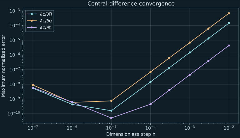
Three derivative errors against step size

Maximum Euclidean error norms
h	cR (1)	cα (m)	ct (m/s)
0.01	1.462e-04	6.896e-04	4.392e-06
0.003	1.316e-05	6.207e-05	3.953e-07
0.001	1.462e-06	6.897e-06	4.392e-08
0.0003	1.316e-07	6.207e-07	3.953e-09
0.0001	1.462e-08	6.897e-08	4.402e-10
1e-05	1.590e-10	7.400e-10	5.055e-11
1e-06	4.279e-10	5.829e-10	6.153e-10
1e-07	5.376e-09	9.002e-09	5.874e-09

2. Regularity and normal

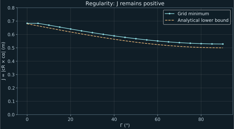
With ρ = R₀ + R cos Γ − W sin Γ, J² = ρ²(1 + WR²) + Wα². For 0 ≤ Γ ≤ π/2 and the parameters above, ρ ≥ 0.68 − 0.18 sin Γ ≥ 0.50 m, hence J ≥ 0.50 m. The parametrization is therefore locally regular throughout this domain for any phases. This does not establish global absence of self-intersections or regularity of the sphere-radius offset surface.

The regularity grid uses 28,224 points per inclination, from 0° to 90° in 5° steps. Maximum normal-length error: 3.33 × 10⁻¹⁶; normalized normal–tangent dot product: 2.18 × 10⁻¹⁶. The J identity agrees numerically to within 1.34 × 10⁻¹⁵ m.

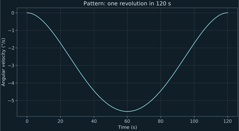
Positive Jacobian throughout the studied family

3. Pattern velocity

For the EN–02 cycle: φₐ(t) = 12π(10u³ − 15u⁴ + 6u⁵), u = t/120. A constant-phase angular coordinate obeys α̇p = −φ̇ₐ/6. Travel is −360°, starting and ending at zero speed. The maximum |α̇p| is 0.09817477 rad/s = 5.625°/s at 60 s. Comparison with finite differences at a 0.001 s step gives a maximum error below 7.95 × 10⁻¹¹ rad/s. This is angular pattern motion, not sphere spin.

Pattern angular velocity over 120 seconds

Data and reproduction

CSV · Convergence · CSV · Regularity · CSV · Pattern · JSON · Study code and data

The package includes instructions to repeat the calculation with Node.js. This verifies the implemented kinematics; dynamics, contact and physical prototype behaviour require separate studies.

03 · Dynamics

Forces, contact, friction and the calculated motion of the sphere.

EN–02 · FIRST NUMERICAL STUDY

One sphere. A 360° cycle.

EN–02 · Numerical dynamic simulation

Study synthesis

Objective: Evaluate circular transport and sphere spin on a prescribed surface.
Method: Homogeneous 1 kg sphere, radius 0.12 m; A = 0.18 m, γ = 0°, μ = 0.15, terrestrial gravity. RK4 with Δt = 0.002 s, compared with 0.001 s.
Results obtained: The reference sphere completes −360° in 120 s and finishes at radius 1.110 m. Minimum normal reaction is 9.810 N. Maximum timestep position difference is 6.04 × 10⁻¹¹ m and maximum energy residual is 1.48 × 10⁻⁷ J.
Scope and limitations: Reference results are for μ = 0.15; changing the control recomputes a different case. Prescribed surface, regularized friction and assumed material coordinates. No experimental calibration or microgravity validation.

A surface at tilt γ = 0° with a sphere initially at rest in a cavity. Normal reaction and tangential friction determine transport and spin. Trajectory and orientation are computed together.

SI example · m = 1 kg · sphere radius = 0.12 m · gravity = 9.81 m/s²

Friction coefficient μ 0.15

Illustrative reference: μ = 0.15, dimensionless. Change it to recompute the cycle; μ = 0 means no friction. This value is not a measurement of the fabric–metal pair.

ViewSurface appearance

Show trajectorySphere-fixed vector

The body-fixed vector starts vertically, normal to the reference XY plane. The arrow and gold band follow the computed sphere orientation; they no longer remain vertical when it spins. With μ = 0 and zero initial spin, orientation stays fixed.

Preparing the trajectory calculation…

The coloured trace shows the computed centre trajectory up to the selected time, projected over the surface for visibility; it is not a contact line on the current membrane.

Contact slip speed—

Friction force—

Cumulative spin—

Sphere spin rate—

Sphere displacement—

Pattern rotation—

Physical time—

Sphere speed—

Normal reaction—

Scrub through the cycle

Download CSV results Parameters and verification

Friction, rotation and numerical method

Illustrative dimensions: R₀ = 0.68 m, R₁ = 2.40 m, A = 0.18 m, Kᵣ = 1, Kₐ = 6. Homogeneous rigid sphere: mass m = 1 kg, radius b = 0.12 m and inertia I = 2mb²/5. Initial conditions are R = 0.43 m, α = π/6, zero velocity and zero spin. Initial orientation is the identity; the body-fixed vector starts at (0, 0, 1).

Geometry has γ = 0° and zero radial phase. Prescribed angular phase is φₐ(t) = 12π(10τ³ − 15τ⁴ + 6τ⁵), with τ = t/120. The pattern completes −360° over 120 physical seconds, with smooth start and stop. Playback at ×8 lasts about 15 seconds.

The centre is X = c + b n. Coordinates (R, α) are assumed to label material surface points; their velocity is ∂c/∂t at fixed coordinates. Slip is the tangential component of V + ω × (−b n) − ∂c/∂t, with V the centre velocity and ω the sphere angular velocity. This material assumption is necessary to define friction.

Regularized Coulomb friction is used: fτ = −μN vslip / √(‖vslip‖² + ε²), with ε = 0.01 m/s. Friction opposes slip and satisfies ‖fτ‖ ≤ μN. Regularization allows small slip speeds; it implements neither exact static sticking nor an imposed pure-rolling constraint.

For q = (R, α), the solver uses (JᵀJ) q̈ = Jᵀ(g + fτ/m − a₀), with J = ∂X/∂q and a₀ the acceleration at constant q̇. Friction torque is (−b n) × fτ and the rotational equation is I ω̇ = (−b n) × fτ. Orientation is integrated as a unit quaternion. Displayed cumulative spin is ∫‖ω‖dt; it is not a net rotation about one fixed axis.

Fourth-order Runge–Kutta integration uses a 0.002 s step. Contact and annular boundaries are checked. The reference case is compared with a 0.001 s step. The energy balance includes translational, rotational and potential energy, surface work and frictional dissipation. Downloaded files match the selected coefficient after calculation.

Surface motion is prescribed and is not deformed by the load; fabric and metal are visual appearances. The reference coefficient and regularized law are assumptions for an exploratory study without experimental calibration. This terrestrial-gravity case does not establish microgravity behaviour.

EN–02R · COUPLED PHASES

One revolution. Radial transport.

EN–02R · Numerical dynamic simulation

Study synthesis

Objective: Combine counterclockwise angular transport and radial motion while retaining EN–02 geometry.
Method: Same physical parameters and initial state; φₐ = −12πs and φᵣ = −πs, with s = 10τ³ − 15τ⁴ + 6τ⁵ and τ = t/120. Dynamic integration and a 0.002/0.001 s timestep comparison.
Results obtained: The sphere completes +360° in 120 s; centre radius increases from 1.110 to 1.970 m. Maximum radial cavity error: 0.901 mm; minimum normal reaction: 9.810 N; minimum radial edge margin: 0.310 m. Maximum timestep difference: 1.61 × 10⁻¹⁰ m; energy residual: 1.49 × 10⁻⁷ J.
Scope and limitations: Contact is maintained in the reference model at μ = 0.15. The path follows from dynamic equations but depends on contact and friction assumptions. Comparison with EN–02 also includes reversing angular direction.

Same geometry, sphere and physical parameters as EN–02. Only the phase laws change: angular motion is counterclockwise viewed from +Z towards the XY plane, and radial phase varies by −π rad to move the cavity outwards.

SI example · m = 1 kg · sphere radius = 0.12 m · gravity = 9.81 m/s²

Friction coefficient μ 0.15

Illustrative reference: μ = 0.15, dimensionless. Change it to recompute the cycle; μ = 0 means no friction. This value is not a measurement of the fabric–metal pair.

ViewSurface appearance

Show trajectorySphere-fixed vector

Preparing the trajectory calculation…

Fixed frame: X × Y = Z, +Z upwards. Positive angular displacement is counterclockwise viewed from +Z. The gold arrow is attached to the sphere; it is not the fixed Z axis.

The coloured trace shows the computed centre trajectory up to the selected time, projected over the surface for visibility; it is not a contact line on the current membrane.

Centre radius—

Radial phase—

Contact slip speed—

Friction force—

Cumulative spin—

Sphere spin rate—

Sphere displacement—

Pattern rotation—

Physical time—

Sphere speed—

Normal reaction—

Scrub through the cycle

Download CSV results Parameters and verification

Friction, rotation and numerical method

Geometry and initial conditions are unchanged: γ = 0°, A = 0.18 m, Kᵣ = 1, Kₐ = 6. With τ = t/120 and s = 10τ³ − 15τ⁴ + 6τ⁵, φₐ = −12πs and φᵣ = −πs. Hence αp = π/6 + 2πs and Rp = 0.43 + 0.86s m. The cavity moves outwards during +360°; these are feature trajectories, not imposed sphere coordinates.

The original EN–02 above is retained unchanged, including its clockwise convention. EN–02R reverses angular phase and adds radial phase. Both start from exactly the same surface and sphere state. This is numerical verification of an idealized terrestrial model, not experimental or microgravity validation.

Reproduce the verification · Node.js

Reference verification (μ = 0.15): +360° in 120 s; centre radius 1.110 → 1.970 m; maximum radial cavity-tracking error 0.901 mm; minimum normal reaction 9.810 N; minimum radial clearance of the sphere envelope to the annular edges 0.310 m. Comparing Δt = 0.002 s and 0.001 s gives a maximum centre-position difference below 2 × 10⁻¹⁰ m; this tests time integration, not all modelling errors.

EN–02 / EN–02R

Compare circular and spiral trajectories

Comparative synthesis: EN–02 approximately retains its radius, while EN–02R increases it by 0.860 m during one revolution. Views share time; opposite angular directions are identified. This is not a third independent simulation.

Synchronized reference cases · μ = 0.15 · original surface and sphere. Circular: EN–02 (clockwise); spiral: EN–02R (counterclockwise). Traces show computed centre paths, not contact points.

ViewSurface appearance

Circular · EN–02

—

Spiral · EN–02R

—

Shared time

Reference data loading when visible.

EN–02 · CSV

Numerical results

Reading EN–02 results: position, velocity, contact, spin and energy from CSV. Charts reflect the loaded dataset or recomputed case; they are not an independent study.

Time histories from the EN–02 CSV for the continuous surface model. Reference case: mass 1 kg, radius 0.12 m, friction μ = 0.15, duration 120 s. These data do not describe the pin mechanism video. Every recorded sample is plotted. Numerical results, not experimental measurements.

Data source Download reference CSV

Loading CSV…

Inspect time

Angular lag = sphere angle − pattern angle; negative angles indicate the chosen direction of travel. Cumulative spin is total angular travel, not final orientation. Energy is plotted relative to its initial value. Each chart has its own vertical scale.

04 · Further research

Reserved for subsequent analytical, numerical and experimental studies.

Planned research areas

No results are claimed for the following areas. Each future study will use the same objective, method, results and limitations structure, with versioned data and reproducible code.

Planned · no results yet

EN–03 · Free-system dynamics

Couple structure and masses; verify angular-momentum balance and attitude response.

Planned · no results yet

Actuation and control

Model force, stroke, bandwidth, power and phase tracking.

Planned · no results yet

Materials and fabrication

Characterize membrane stress, fatigue, tolerances and actuator integration.

Planned · no results yet

Experimental validation

Define tests, sensors, uncertainty and quantitative model/prototype comparisons.

Planned · no results yet

Aerospace integration

Study microgravity confinement, interfaces and demonstrator requirements.